With Erasure Coding we can shrink write-cold data even more to have less used space on the extend store. I’m not going to explain how this works as Nutanix has done a great job explaining this already (Link, Link). In this blog post I want to show when Erasure Coding kicks in and how much data reduction I got.
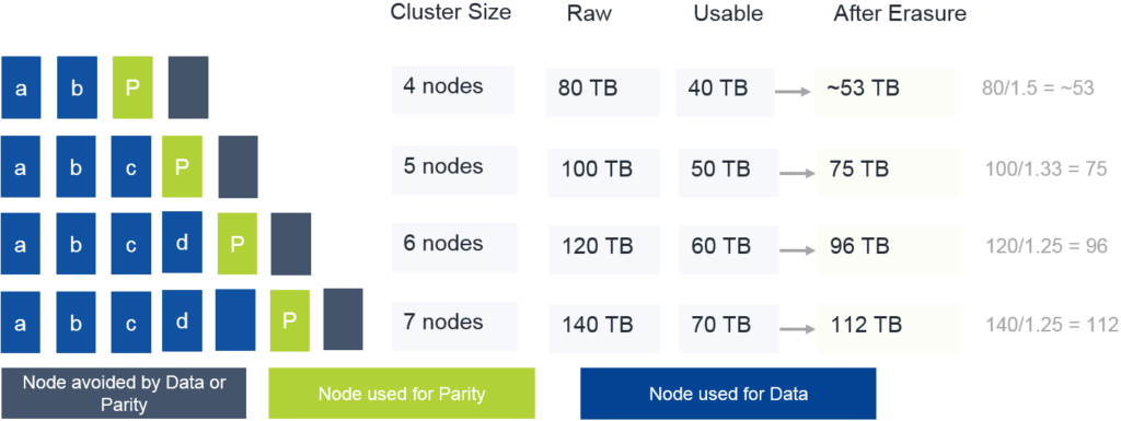
My lab is a 4 node cluster (which is the minimum nodes to enable Erasure Coding) so I will have a saving approximately 25%. This is because I have a strip size of 2/1 (2 data blocks and 1 parity block) and off course 1 empty block for the rebuild.
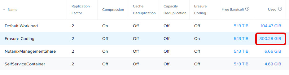
Lets put this to the test. I have created the following storage container:
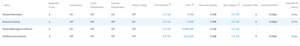
The “Erasure-Coding” storage container is create with no storage optimisation enabled except Erasure Coding.
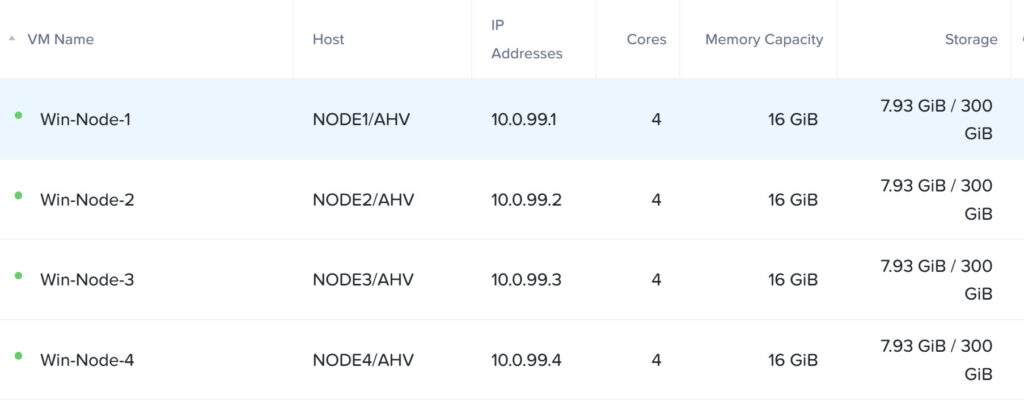
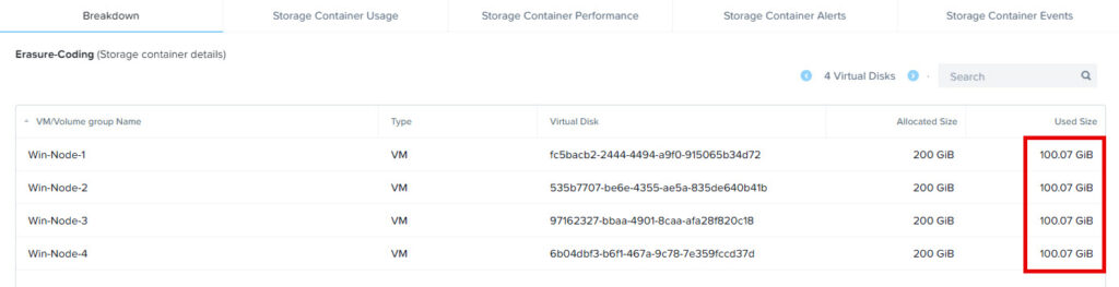
There are 4 Windows virtual machine created with their bootdisk (100GB) on the default workload container and a 200GB data disk on the erasure coding storage container:
Then I generated 100GB of random data on each virtual machine on the disk which is on the erasure coding enabled storage container:
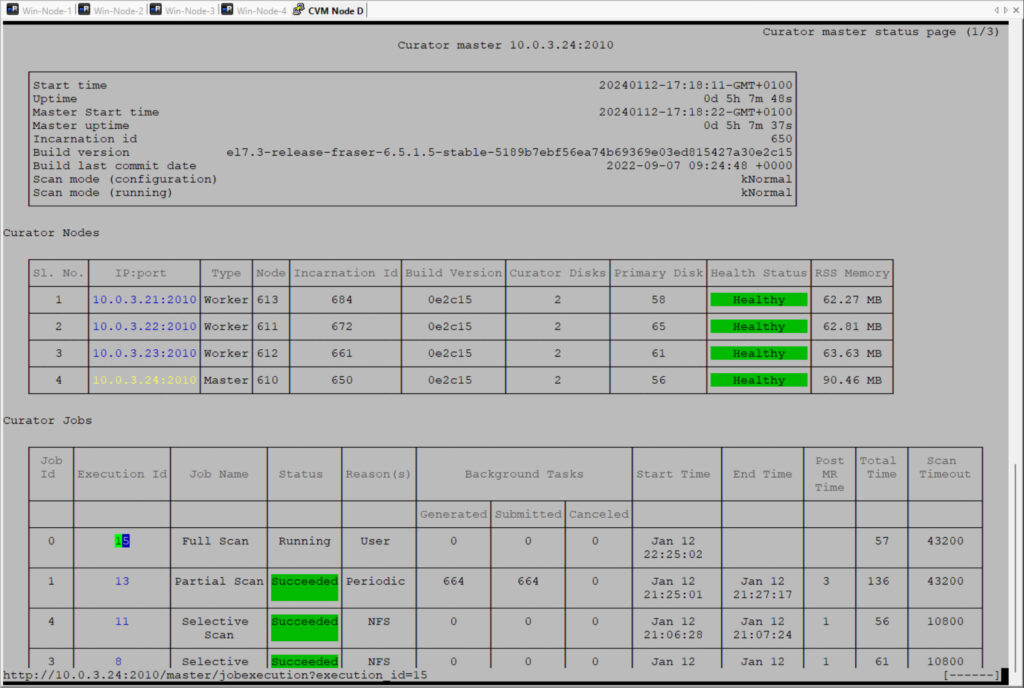
I’ve waited a full curator scan to be sure storage optimalisation is up to data 😉
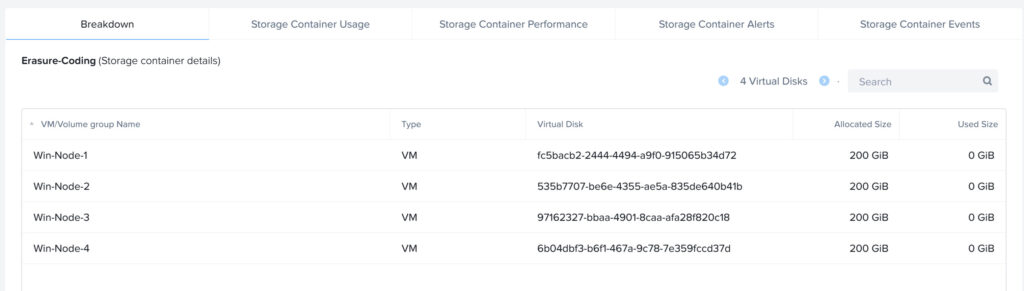
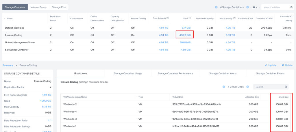
As you can see in the screenshot the actual data is still 400GiB on the Storage Container:
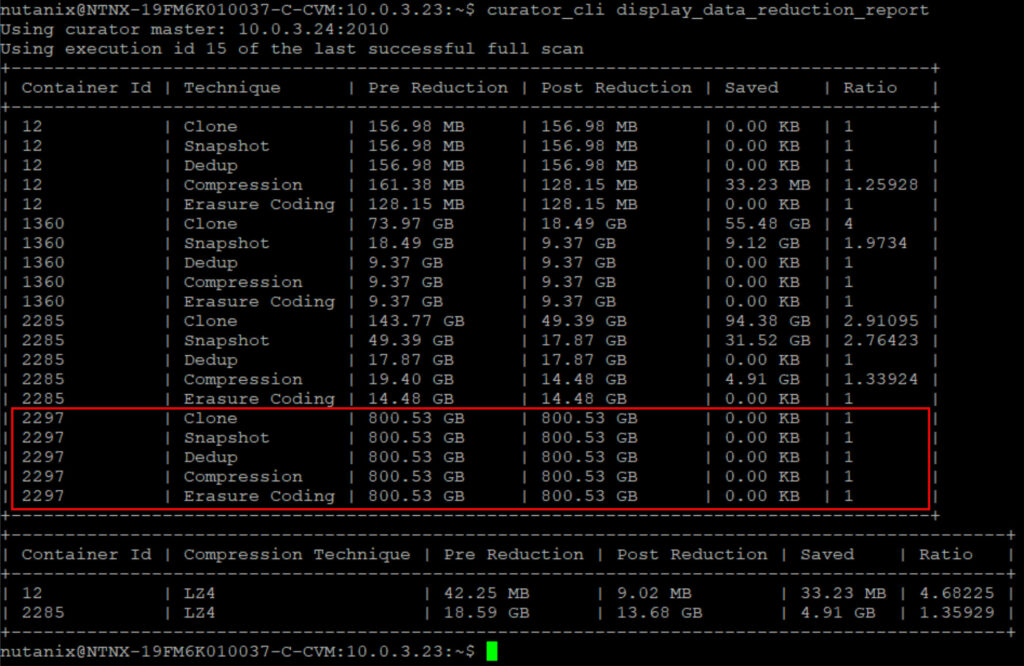
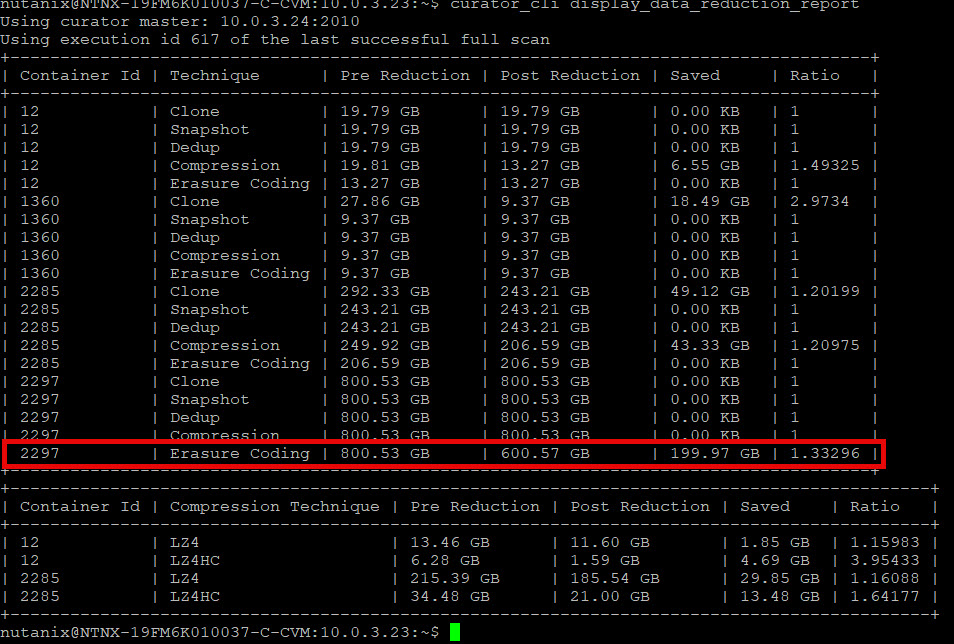
And to be more specific the curator reduction report is also showing the same numbers (800GB as this is the raw data, as I’m running Replication Factor 2).
Now lets wait for 7 days. To see what erasure coding is doing with the data.
And the curator data reduction report looks like this:
Please keep in mind that erasure coding is only for specific type of workloads, for example:
- Write once, read many (WORM) workloads;
- Backups;
- Archives;
- File servers;
- Log servers;
- Email (depending on usage).


Hello, Jeroen,
Why the Ratio is 1.33? You have 4 nodes and according documentation it should be 1.5 isn’t it? YOu have four nodes-2 data+1 parity+1 standby. So it should be 1.5 and 800/1.5 should be 533 gb. Dont understand. In case of 5 nodes its correct, but you don’t have 5 nodes.
Thank for the answer in advance
No it is correct. So in the blogpost on the top you see a table which has a four node example as well. Usable 40TB with EC is is 53TB. That is 33% increase. But yeah the 1.33 should be written like 33% ;)\
And in my case I got 600Gb witten of the actual 800GB. So 600GB + 33% = 800GB. I know it is a bit misleading, but you can to calculate the other way around.
Thank you for your answer, Jeroen. But i am still confused with the calculations.
You have 4 nodes cluster – each contains 100 GB data in container with EC. Its 800 GB RAW -its ok. So the usable is 400 GB. So according the blogpost on the top and according the table with 4 nodes configuration 800/1.5=should 533. Why its 600 instead of 533 like you have 3+1 and not 2+1 EC configuration?
Thanks
In the lab I have this running on a 4 node cluster. And the top screenshot comes from the Nutanix bible.
My savings are 25%. 800GB-25%=600GB. Correct?
If you calculate it the other way around (600GB+33%=800GB) then it is 33%. This is what the cli is using. That is the 1.33.
They greyed out 1.5 in the top screenshot has nothing to do with the savings percentage. Don’t get miss leaded with that.
Got it.
So in case of 4 nodes i will have 50 percent overhead compared to inital data-so in case of 400 gb i will have 600 gb data with EC parity. And compared to RF2 its 33 percent difference=800/6001=1.33 -correct.
Incase of 4 node EC parity is 50%
5 nodes-33% (3 data+1 parity+1 standby)
6 nodes and more -25 percent
Am i correct?
Thanks